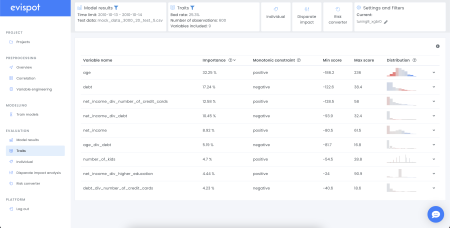
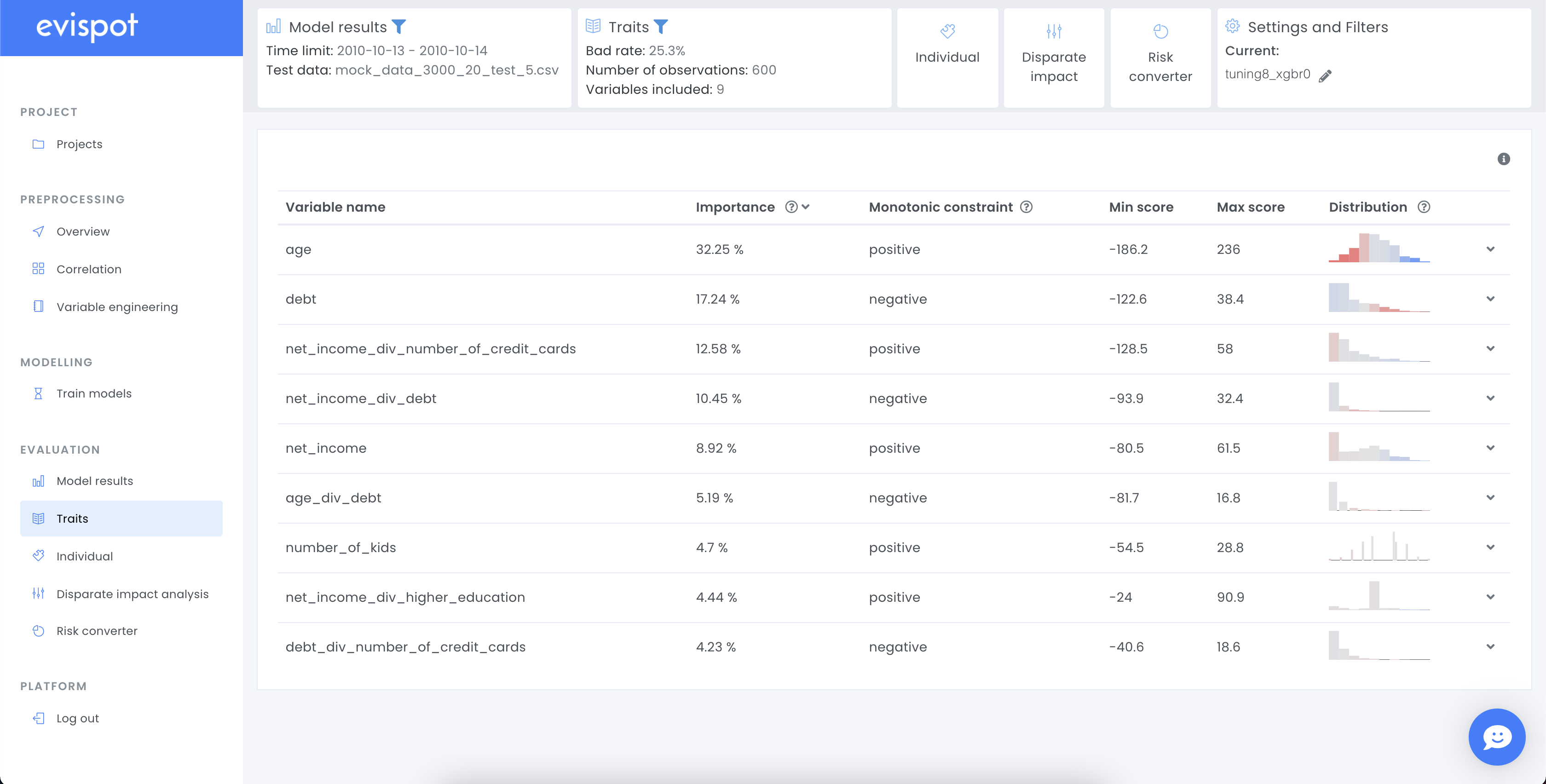
Traits
The traits view displays a table including all variables that were used when training a model. Apart from the variable name, an importance column, monotonic constraint, max, min and distribution plot can be seen. The columns importance, min max and the colour in the distribution plot are based on research approved transparency technique, shapley values. It is possible to further study each variable individually by expanding a variable clicking on the arrow to the right side.
Variable analysis
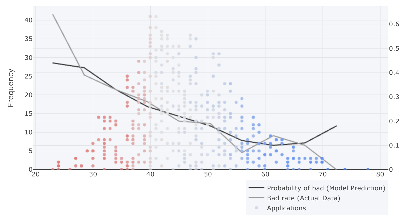
The detailed variable plot will show you a detailed view of the variable.
X-axis: Represents the variable’s value. In the example above it can be seen that the variable has values between 20 – 75 years old.
Left Y-axis: Represents the number of variable observations (Frequency). In the example above it can be seen that the majority of observations are between 40 and 50.
Color of observations (Left Axis): Represent a color scale from red – grey – blue, where red has a negative effect on the score (high risk), grey has no effect on the score (no risk) and blue has a positive effect on the score (low risk).
Right Y-axis: Represent a number between 0 – 1, illustrating the probability of an event occurring.
Colour of lines (Right Axis): The black line represents the model’s prediction, the probability of bad. The grey line represents the number of bads in the actual data.
Variable interaction analysis
The variable interaction analysis plot will show you the contributed impact two variables have together. Ordered so the variable with the most interaction (average of all applications) is listed at the top, while the variable with least interaction will be at the bottom. IT will only be possible to analyse variables that are interacted with each other.
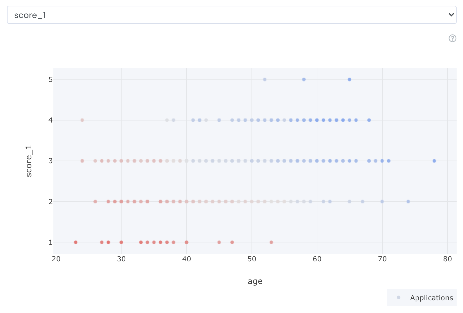
Y-axis: Represent the variable value from the dropdown menu: In the example above it is score_1.
X-axis: Represent the variable value we chose to analyze. In the example above it is age.
Partial dependence plot
The below partial dependence plot represents a nonlinear relationship. If a constraint had been added to the model the blue line would have been forced to go into one direction (e.g always lower score the higher variable value or higher score the higher variable value.)
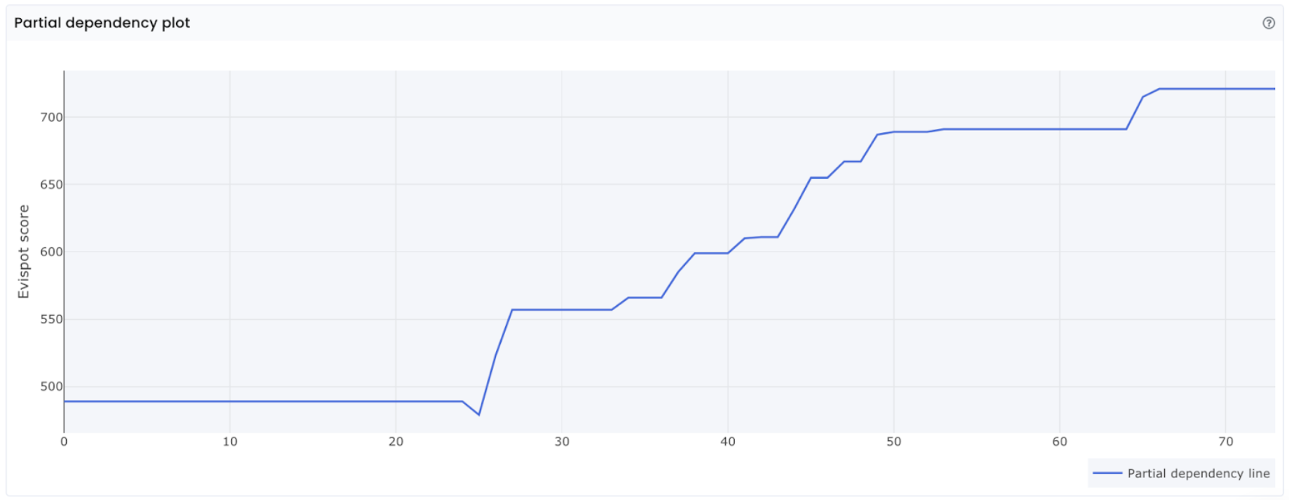
X-axis: Represent the variable value we chose to analyze
Y-axis: Represent the Evispot score.
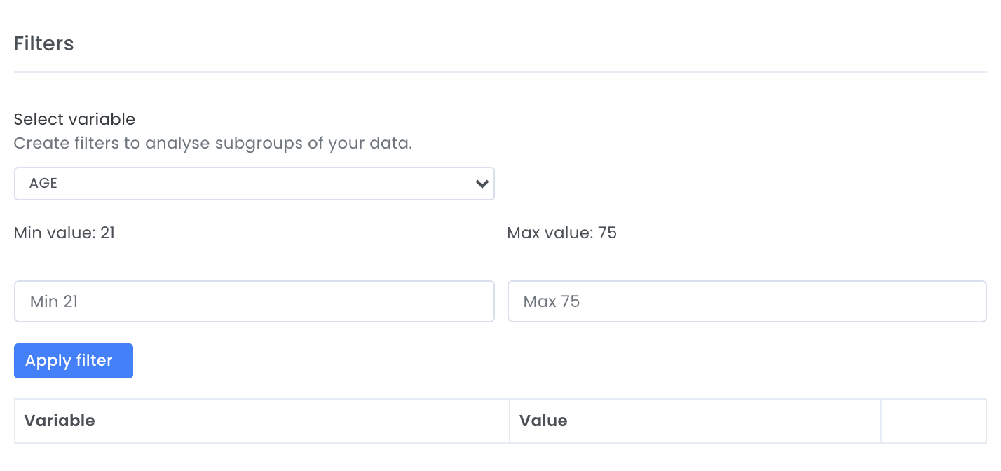
Segmenting and filtering the test data
It is possible to filter and segment the test data to analyse subgroups of the test data more thoroughly. It is possible to filter data based on date interval, numerical values or categorical values. An example could be if a personal credit decision model is built and you want to analyse people under a certain age or if a portfolio analysis model is built and you want to analyse all data points where a person/company has been late with a payment. If a filter is set, the evispot AI platform will recalculate; score based results, Out-of time based results, cross-validation results, distribution plots and traits.
We exist to ensure that decisions are given in an accurate, transparent, ethical & fair manner.
