The preprocessing view visualizes the uploaded data set in many different ways. General information about the data set such as, number of rows, number of variables, number of bad and good. The Evispot AI platform has also calculated statistics and plots for each variable to ease the data analyse process. Two types of preprocessing can be created, regular preprocessing and automatic feature engineering preprocessing.

Regular preprocessing

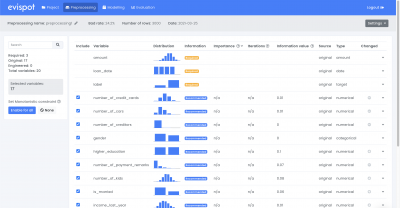
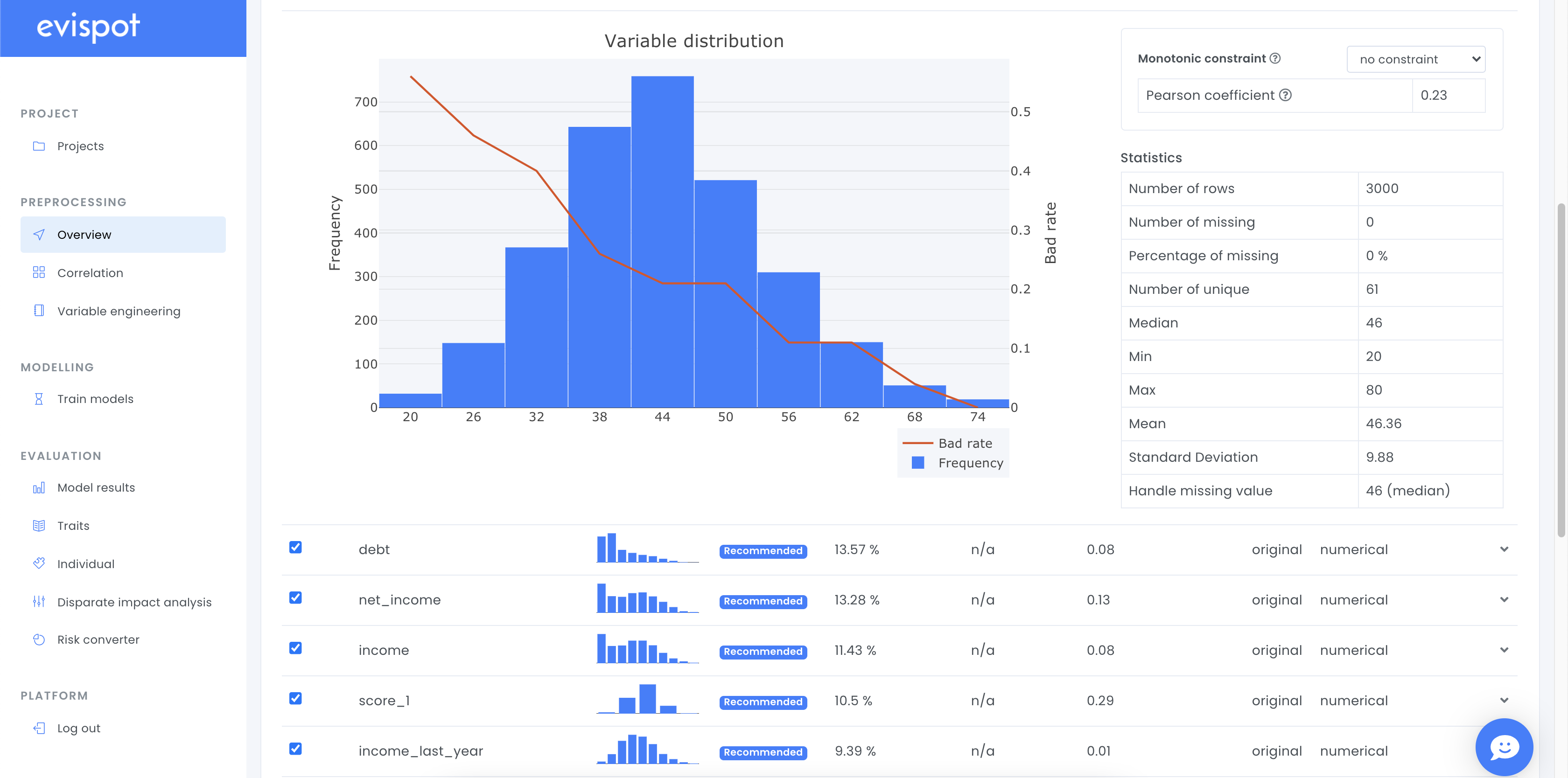
After a project has been created the software creates a regular preprocessing from the uploaded data and displays detailed information about each variable in a table.

Each row in the column displays information about one variable, such as name, distribution plot, variable type and information value. More statistics about each variable such as the number of missing values or detailed distribution plot with bad rate can be found if a variable is expanded, using the arrow to the right. 

Variable engineering

Automatic variable engineering is started when a user creates a new preprocessing by clicking on the button Run Variable Engineering in view preprocessing settings view. This means that the Evispot AI platform will automatically do feature engineering and feature selection.

When automatic feature engineering has been finalized, additional information about each variable will be available, such as importance score, iteration for both the original data that was uploaded and the engineered variables that were created. The software will show, which variables the software recommends to use during model training. However, the user will always be in charge by choosing the variables that will be included in the training model view. (for more information see What is happening under the hood.)

As per the OXFORD dictionary, monotonic is a function or quantity varying in such a way that it either never decreases or never increases. A positive constraint means that for an increasing variable value it´s contribution to the score will be positive. A negative constraint will mean the opposite. A more concrete example could be if a credit decision model is developed. If everything else is equal, it is expected that a person with higher salary will have a lower probability of default compared to a person with lower salary. However if there are some applications in the data having the reversed relationship, higher salary associated with more defaults, that are counter-intuitive. This kind of situation often happens if data is sparse or has a lot of noise. 

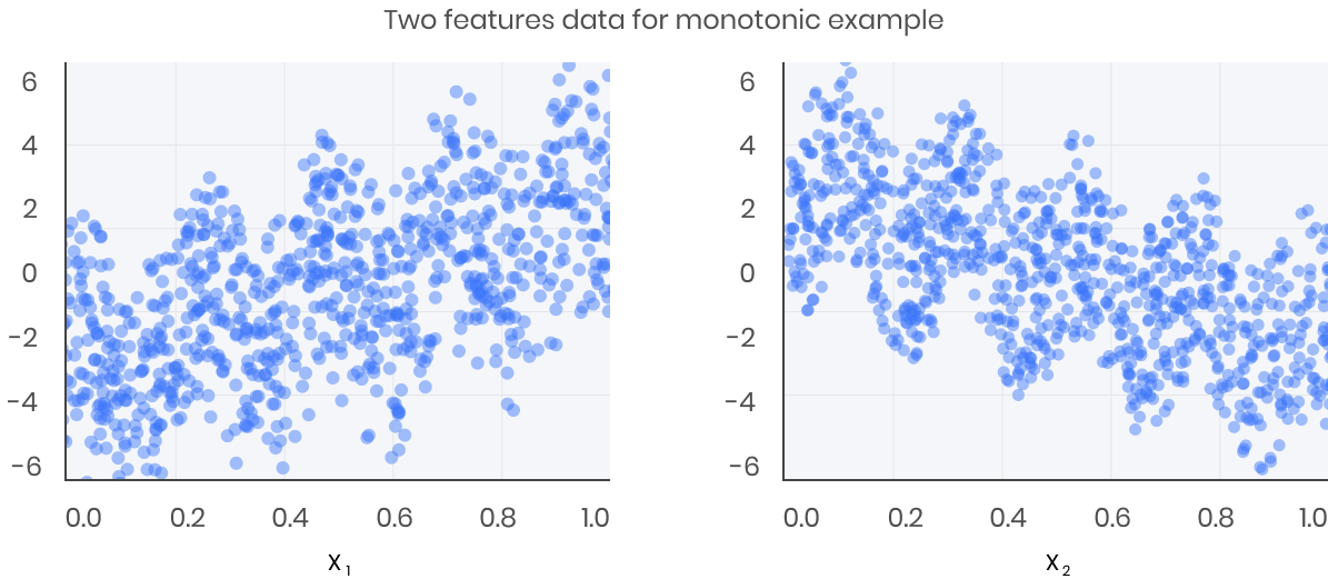
To illustrate, let’s create some simulated data with two features and a response according to the following scheme

The response generally increases with respect to the x1 feature, but a sinusoidal variation has been superimposed, resulting in the true effect being non-monotonic. For the x2 feature the variation is decreasing with a sinusoidal variation.

Let´s fit a model to this data without imposing any monotonic constraints

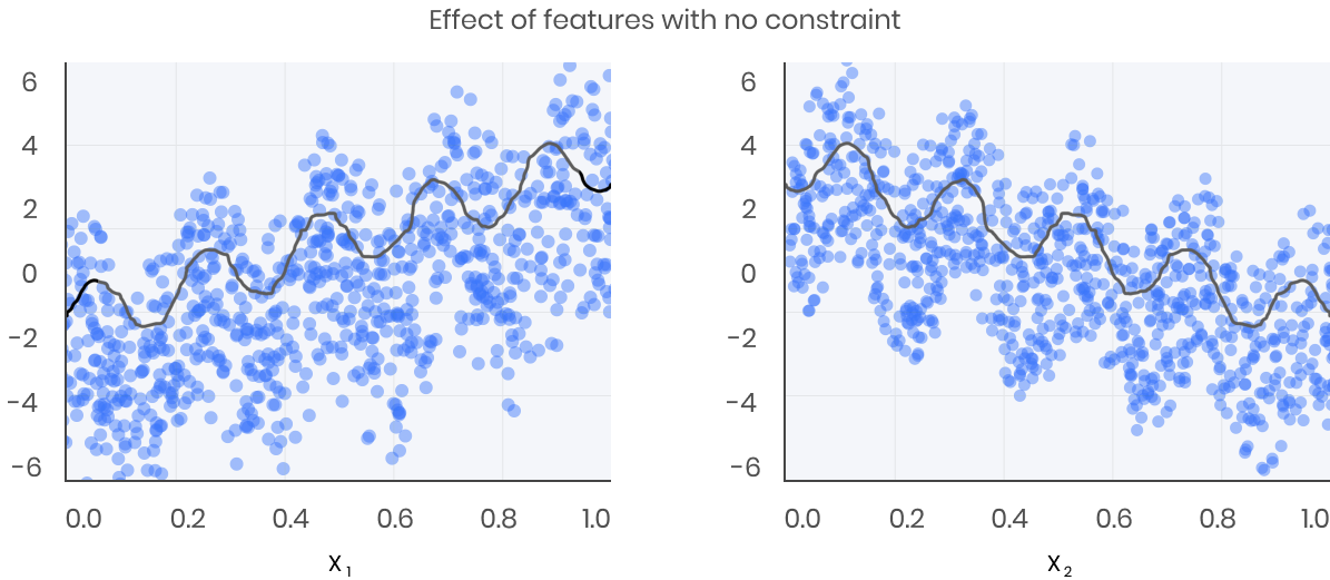
The black curve shows the trend inferred from the model for each feature. To make these plots the distinguished feature xi is fed to the model over a one-dimensional grid of values, while all the other features (in this case only one other feature) are set to their average values. We see that the model does a good job of capturing the general trend with the oscillatory wave superimposed.

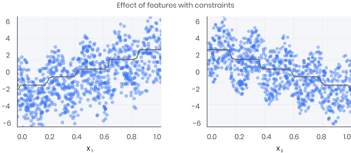
Here is the same model, but fit with monotonicity constraints:

If you as a modeler or your team has experience and know-how within the field you are operating in, setting a variable constraint can often result in better model performance on the test data, meaning that the constrained model may generalize better compared to not using any constraints. Another advantage using monotonic constraint is that the model will be easier to trust and understand.

To be able to train and analyse a transparent monotonic model, constraints must be supplied. The constraint should determine whether the learned relationship between an input variable and the target will be increasing for increases in an input variable or decreasing for increases in an input variable. A metric that can be used to determine the constraint is the pearson coefficient. The Pearson coefficient measures the correlation between the variable and the target. It returns a value between -1 and 1, where 1 indicates a strong positive correlation, -1 a strong negative and 0 indicates no correlation. Hence, a positive pearson coefficient will result in a positive constraint and a negative pearson coefficient will result in a negative constraint. 

There are two ways to set a monotonic constraint in the evispot AI platform, either by expanding the preprocessing table and adding the constraint for one variable at a time. Another alternative is to set monotonic constraint on all variables automatically, using the variables Pearson Coefficient value.

A common tool to evaluate if a monotonic constraint has been set to a model is by looking at a partial dependence plot, which can be found in the evaluation view after a model has been trained in view Evaluation section Traits.